Excel VLOOKUP Explained: Step-by-Step Example
How to Use VLOOKUP in Excel (Step-by-Step Example)
VLOOKUP is one of Excel’s most commonly used formulas. It allows you to search for a value in a table and return related data from another column in the same row.
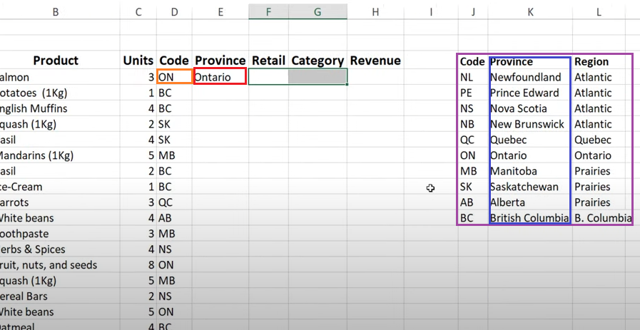
In this example, we will use VLOOKUP to convert a province code into a full province name.
The VLOOKUP Formula in this Example
=VLOOKUP(D4,$J$3:$L$13,2,0)The VLOOKUP formula was entered in cell E4.
Breaking Down the Formula
Each part of the formula has a specific purpose:
D4
The cell that contains the value you want to look up.
In this example, D4 contains the value ON, which is the province code we want to translate into a full name.
$J$3:$L$13
The table array. This is the range of cells where Excel will search for the lookup value.
- Column J contains the province codes
- Column K contains the province names
- Column L contains the region names
The dollar signs lock the range so it does not move if the formula is copied to other cells.
2 = Column index Number
The column index number.
This tells Excel which column from the table array to return data from:
- Column 1 = J (Code)
- Column 2 = K (Province)
- Column 3 = L (Region)
Because we want the province name, we use 2.
0 – zero in the formula
The match type.
- 0 = Exact match
- 1 = Approximate match
Since province codes must match exactly, we use 0.
How the Formula Works
- Excel looks at the value in D4, which is ON.
- It searches for ON in the first column of the table range J3:J13.
- Excel finds ON in cell J9.
- Because column index 2 was specified, Excel returns the value from the second column of that row.
- The value in K9 is Ontario.
- Ontario is displayed as the result in cell E4, where the VLOOKUP formula was entered.